Constraint Solving in jaxCAD

solve_constraints finds parameter values that satisfy all geometric constraints attached to a scene. It errors immediately if the system is under- or over-constrained, so you never silently get a wrong result.

import jax.numpy as jnp
import matplotlib.patches as patches
import matplotlib.pyplot as plt
import numpy as np

from jaxcad import extract_parameters, functionalize
from jaxcad.constraints import DistanceConstraint, solve_constraints
from jaxcad.geometry import Vector
from jaxcad.render import render_raymarched
from jaxcad.sdf import Sphere, Translate

Scene setup - trilateration

Three anchor points at known positions and one unknown point p. We give p a deliberately wrong initial guess - the solver will find the true position.

• Anchors are fixed (free=False) - they are known constants.
• p is free (free=True) - the unknown we want to solve for.

We also define true_p = [2, 1, 0] - the intended solution - so we can compute exact target distances.

anchor_a = Vector(jnp.array([0.0, 0.0, 0.0]), free=False, name="anchor_a")
anchor_b = Vector(jnp.array([4.0, 0.0, 0.0]), free=False, name="anchor_b")
anchor_c = Vector(jnp.array([2.0, 3.0, 0.0]), free=False, name="anchor_c")

true_p = jnp.array([2.0, 1.0, 0.0])  # the answer we want the solver to find

p = Vector(jnp.array([0.5, 0.5, 0.0]), free=True, name="p")  # wrong initial guess

scene = Translate(Sphere(radius=0.5), offset=p)

Each distance constraint is a circle centered on an anchor with radius equal to the distance from that anchor to true_p. The solver finds where all three circles intersect.

anchors = {
    "A": np.array([0.0, 0.0]),
    "B": np.array([4.0, 0.0]),
    "C": np.array([2.0, 3.0]),
}
true_xy = np.array([2.0, 1.0])
guess_xy = np.array([0.5, 0.5])

fig, ax = plt.subplots(figsize=(5, 5))

for _name, pos in anchors.items():
    r = np.linalg.norm(true_xy - pos)
    ax.add_patch(
        patches.Circle(
            pos, r, fill=False, linestyle="--", linewidth=1.2, color="steelblue", alpha=0.5
        )
    )

for name, pos in anchors.items():
    ax.plot(*pos, "s", color="steelblue", markersize=10, zorder=5)
    ax.annotate(f"anchor {name}", pos, textcoords="offset points", xytext=(8, 4), fontsize=9)

ax.plot(
    *guess_xy,
    "x",
    color="orange",
    markersize=12,
    markeredgewidth=2.5,
    zorder=5,
    label="initial guess  (0.5, 0.5)",
)
ax.plot(*true_xy, "o", color="crimson", markersize=10, zorder=6, label="true p  (2, 1)")

for pos in anchors.values():
    ax.plot(
        [pos[0], true_xy[0]],
        [pos[1], true_xy[1]],
        "--",
        color="steelblue",
        linewidth=0.8,
        alpha=0.4,
    )

ax.set_xlim(-1.5, 6)
ax.set_ylim(-1.5, 5)
ax.set_aspect("equal")
ax.legend(loc="upper right", fontsize=9)
title = "Trilateration problem setup\n(dashed circles = distance constraints)"
ax.set_title(title, fontsize=10)
ax.set_xlabel("x")
ax.set_ylabel("y")
plt.tight_layout()
plt.show()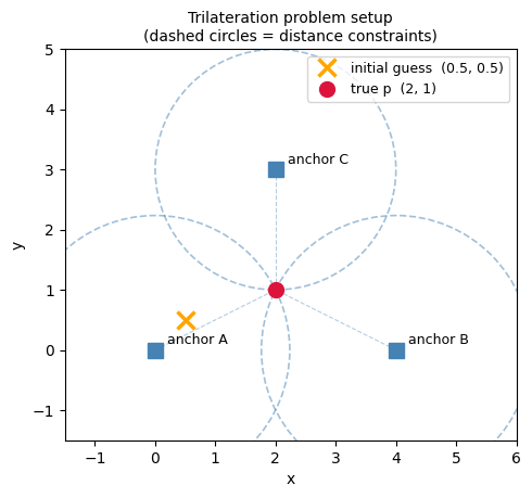

Degrees of freedom

p is a 3D Vector → 3 DOF. Each DistanceConstraint enforces one scalar equation → removes 1 DOF. We need exactly 3 constraints to reduce to 0 remaining DOF and uniquely solve for p.

Under-constrained error

Adding only one constraint leaves 2 DOF - solve_constraints raises a clear error.

DistanceConstraint(p, anchor_a, float(jnp.linalg.norm(true_p - anchor_a.value)))

try:
    solve_constraints(scene)
except ValueError as e:
    print(e)

Under-constrained: 2 DOF remaining. (3 parameter DOF, 1 constraint equations)

Fully constrain the scene

Add the remaining two constraints - one per anchor - each with the exact distance from true_p to that anchor.

DistanceConstraint(p, anchor_b, float(jnp.linalg.norm(true_p - anchor_b.value)))
DistanceConstraint(p, anchor_c, float(jnp.linalg.norm(true_p - anchor_c.value)))

DistanceConstraint(p, anchor_c, d=2.0)

Solve

solve_constraints runs Levenberg-Marquardt (via optimistix) starting from the wrong initial guess (0.5, 0.5, 0) and converges to the true position (2, 1, 0).

free_params, fixed_params, metadata = extract_parameters(scene)
solved_params = solve_constraints(scene, max_steps=10)

print("Initial p: ", p.value)
print("Solved p:  ", solved_params["p"])

Initial p:  [0.5 0.5 0. ]
Solved p:   [1.9999999 0.9999999 0.       ]

Render at the solved position

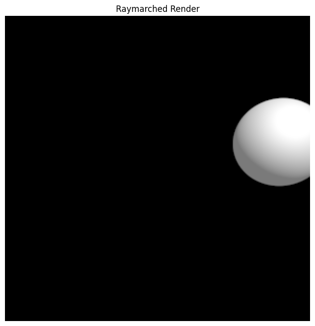
The solved parameter dict is drop-in compatible with functionalize, so the constrained scene slots directly into the optimization workflow.

render_raymarched(
    functionalize(scene)(solved_params, fixed_params),
    camera_pos=jnp.array([3.0, 2.0, 3.0]),
    resolution=(300, 300),
    aa_samples=2,
)